A Look at the 3-SAT Phase Transition

Posted on April 21, 2019 by Erik Davis

Tags: math, computational-complexity, 3-SAT

Introduction

There’s a classic problem in theoretical computer science, 3-SAT, which asks whether a Boolean expression in “conjunctive normal form” can be satisfied. The ‘3’ in the name means that each clause involves at most three variables or their complements. For example:

(w or y or not z) and (x or not z or y)

is a Boolean expression with two clauses, each of which contains three variables from w,x,y,z. We will sometimes refer to such an expression as a 3-SAT “instance”.

If, given a Boolean expression like the one above, we can find an assignment of True or False to each variable that satisfies all of the clauses together, then the expression is “satisfiable”. It’s known that this decision problem is NP-complete, and so being able to solve it “efficiently” would mean that you could solve other hard problems, like the Traveling Salesman Problem, “efficiently”.

With that said, it’s pretty easy to find a satisfying assignment for the Boolean expression we wrote above, because there are 4 variables total and only 2 clauses. Even with dumb guessing, you will stumble into a solution pretty quickly. For example, if I pick y=True then the above expression is satisfied regardless of the choices for w,x,z. There just simply aren’t enough constraints to make things difficult.

If, on the other hand, we had written down a list of 100 clauses, built from the same variables w,x,y,z, it’d be rather unlikely that there’s any satisfying assignment. A few clauses are no big deal, but given enough we’d expect some sort of conflict to arise.

Generating 3-SAT instances

Let’s play around with this idea a bit. With the code below we can cook up random 3-SAT clauses.

import random

def random_clause(vars):
    """Return a random 3-SAT clause."""

    clause_vars = random.choices(vars, k=3)
    modifiers = random.choices(["", "not "], k=3)
    exprs = [f"{v}{x}" for x,v in zip(clause_vars, modifiers)]
    clause = " or ".join(exprs)
    return clause

>>> random_clause("wxyz")
'not w or not z or w'

From this, we can generate random 3-SAT problems. Here I’m going to represent a 3-SAT instance with \(n\) variables as a Python function of \(n\) parameters.

def random_3sat(num_vars, num_clauses):
    """Return a random 3-SAT instance.

    The resulting problem is represented as a Python function,
    with `num_vars` arguments. When applied to `num_vars` Boolean values,
    the function returns True if they constitute a satisfying assignment.
    """

    vars = [f"x_{i}" for i in range(num_vars)]

    clauses = ["(" + random_clause(vars) + ")" for _ in range(num_clauses)]

    body = " \\\n and ".join(clauses)
    header = "lambda " + ",".join(vars) + ": \\\n"
    problem = eval(header + body)
    problem.num_vars = num_vars
    return problem

So, for example, we can get a problem with 4 variables and 2 clauses:

>>> prob = random_3sat(4, 2)
>>> print(prob)
<function <lambda> at 0x12b30e7b8>

>>> prob(True, True, True, True)
True

Although using a lambda to represent problems is a bit opaque, the main thing we will be doing with them is checking whether an assignment satisfies them. Creating a function for this is the naive way of making this check fast. You can get a sense of how lightweight this is by just checking the bytecode:

>>> from dis import dis
>>> dis(prob)
  2           0 LOAD_FAST                0 (x_0)
              2 UNARY_NOT
              4 POP_JUMP_IF_TRUE        16
              6 LOAD_FAST                2 (x_2)
              8 POP_JUMP_IF_TRUE        16
             10 LOAD_FAST                3 (x_3)
             12 UNARY_NOT
             14 JUMP_IF_FALSE_OR_POP    28

  3     >>   16 LOAD_FAST                0 (x_0)
             18 JUMP_IF_TRUE_OR_POP     28
             20 LOAD_FAST                0 (x_0)
             22 JUMP_IF_TRUE_OR_POP     28
             24 LOAD_FAST                1 (x_1)
             26 UNARY_NOT
        >>   28 RETURN_VALUE

With this in mind, let’s also implement the dumbest naive method of checking satisfiability: brute force.

from itertools import product

def satisfy(problem):
    """Find a satisfying assignment for a given 3-SAT problem.

    Returns a tuple of truth values, or None if no satisfying 
    assignment exists.
    """

    for assignment in product([True, False], repeat=problem.num_vars):
        if problem(*assignment):
            return assignment
    return None

With this we can easily recover an assignment:

>>> satisfy(prob)
(True, True, True, True)

You can try it out and observe that there’s a lower chance of being satisfiable if we add more clauses:

>>> bigger_prob = random_3sat(4, 100)
>>> satisfy(bigger_prob)
# None

Getting a Bird’s Eye View

Now that we have a way to generate “random” 3-SAT instances, let’s see how the probability that one such instance is satisfiable varies with the number of clauses. To do this, we’ll consider for now a fixed number of variables, and several values of num_clauses we’ll generate some 3-SAT instances and check whether they are satisfiable.

import pandas as pd

def sat_experiment(num_vars, clause_range, sample_size=20):
    """Generate a number of random 3-SAT instances and tries to satisfy them.

    Returns a Pandas dataframe with three columns: 'num_vars', 'num_clauses',
    'satisfiable'. Here 'satisfiable' is a proportion (between 0 and 1), as
    observed over a finite sample.
    """

    data = []
    for num_clauses in clause_range:
        for i in range(sample_size):
            prob = random_3sat(num_vars, num_clauses)
            satisfiable = 1.0 if satisfy(prob) is not None else 0.0
            data.append([num_vars, num_clauses, satisfiable])
    df = pd.DataFrame(data, columns=['num_vars',
                                     'num_clauses',
                                     'satisfiable'])
    df = df.groupby(['num_vars', 'num_clauses'], as_index=False).mean()
    return df

As a brief example, consider the following, which generates a random 3-SAT problem with 4 variables and 5, 10, …, 50 clauses, and then checks whether it is satisfiable. Here a 1.0 means that the problem is satisfiable, a 0.0 means that it is not.

>>> sat_experiment(4, range(5, 50, 5), sample_size=1)
   num_vars  num_clauses  satisfiable
0         4            5          1.0
1         4           10          1.0
2         4           15          1.0
3         4           20          1.0
4         4           25          0.0
5         4           30          0.0
6         4           35          0.0
7         4           40          0.0
8         4           45          0.0

Of course, the hard cutoff from 1.0 to 0.0 that we see there is something of an artifact; if we had considered more samples we’d expect a more gradual transition (with a bit of noise, since we’re estimating the true proportions by sample means):

>>> sat_experiment(4, range(5, 50, 5), sample_size=20)
   num_vars  num_clauses  satisfiable
0         4            5         1.00
1         4           10         1.00
2         4           15         0.85
3         4           20         0.80
4         4           25         0.55
5         4           30         0.15
6         4           35         0.05
7         4           40         0.00
8         4           45         0.10

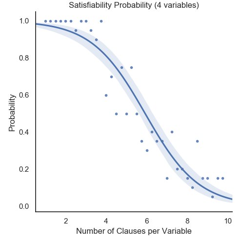
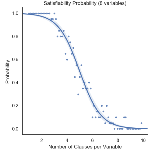
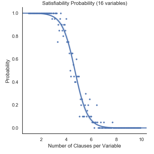
From now on, we’ll just visualize this data by plotting it and fitting a curve. We now also consider how things change as we increase the number of variables. In order to put things on a common scale, we consider the number of clauses per variable on the \(x\)-axis below. Here are pictures for 4, 8, and 16 variables.

The Phase Transition

All three of the pictures show a similar phenomena: the probability that a 3-SAT instance can be satisfied starts at nearly \(1\), when there is only a single clause per variable, and drops off to nearly \(0\), when there are sufficiently many clauses per variable. But if you pay close attention, you will observe two other interesting features.

First, the transition from \(1\) to \(0\) occurs at a similar place in each plot.
Second, the sharpness of the transition seems to increase as the number of variables increases.

If, for example, both of these held true as we increased the number of variables to infinity, one would ultimately expect a plot like this:

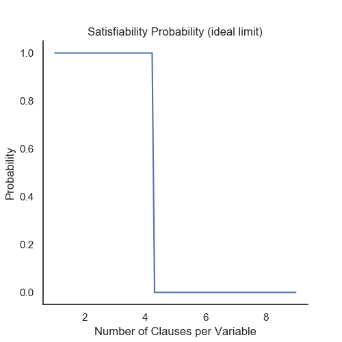
In the language of physics, a phase transition. Informally speaking, a phase transition is when there is an abrupt change in the properties of a system under a gradual change of some macroscopic variable. The most classic example is the freezing of water: as the temperature decreases, there is an abrupt transition of from a “liquid phase” to a “solid phase”. But in fact there are many other examples of phase transitions. One of the most remarkable demonstrations is of the “Curie Point”, the temperature at which iron spotaneously gains or loses its ferromagnetic properties.

Let’s work out the analogy with 3-SAT here.

	Water	3-SAT
Size of the system	Number of molecules	Number of variables
Phases	Solid vs Liquid	Unsolveable vs Solveable
Macroscopic Variable	Temperature	Variables per Clause

Summary

So, we made some plots and then a vague analogy with water freezing. But does 3-SAT really exhibit a phase transition?

The short answer is yes. We could have demonstrated stronger evidence for this by considering a larger number of variables (although, in this case it would also be a good idea to implement something like a backtracking solver, rather than brute force).

The long answer is that, in terms of the theoretical understanding of things, some of the mathematical issues are still open. I won’t go into technicalities too much here, but as far as I know (e.g. based on this question), the current state of understanding is this:

There is rigorous mathematical work proving something slightly weaker than the existence of a phase transition for \(k\)-SAT with \(k=3\).
Physicists have worked out what the threshold should be: roughly 4.2667 clauses per variable.
The analogous result for large values of \(k\) has been proved rigorously. This, together with the other evidence, gives strong support for the behavior of \(k=3\).

References

For the code in this article, look here. For more information about this phenomena, see Chapter 14 of Moore and Mertens, The Nature of Computation.