An Introduction to Continued Fractions

Posted on July 31, 2016 by Erik Davis

Tags: number-theory, continued-fractions, haskell

Continued fractions offer a representation of numbers distinct from the more common decimal expansion. This representation can be finite, as in \[ \frac{10}{7} = 1 + \cfrac{1}{2 + \cfrac{1}{3}},\] or infinite, as in \[ \varphi = 1 + \cfrac{1}{1 + \cfrac{1}{1 + \cfrac{1}{1 + \ddots}}},\] where $\varphi = \frac{1+\sqrt{5}}{2}$ is the golden ratio.

The study of continued fractions has fascinated mathematicians for millenia. For example, they are intimately connected with certain mysterious approximations ¹, such as \[ \pi \approx \frac{355}{113} = 3.1415929\ldots.\] In this article, we mention some basic results in the theory of continued fractions, focusing our attention on finite continued fractions. In subsequent articles we will take up the more general case of infinite continued fractions, and discuss some applications of the theory.

We demonstrate some of the ideas involved through Haskell code. The reader is encouraged to follow along and experiment on their own.

Notation

For what follows, we consider only continued fractions with ones in the numerator, and with addition in the denominator. Thus we will not be considering generalized continued fractions, such as \[ \tan(x) = \cfrac{x}{1 - \cfrac{x^2}{3 - \cfrac{x^2}{5 - \cfrac{x^2}{7 - \ddots}}}}. \]

We will abbreviate the continued fraction \[ a_0 + \cfrac{1}{a_1 + \cfrac{1}{\ddots \, + \cfrac{1}{a_N}}} \] by $[a_0,a_1,\ldots,a_N]$, and similarly \[ a_0 + \cfrac{1}{a_1 + \cfrac{1}{a_2 + \ddots}} \] by $[a_0,a_1,a_2,\ldots]$. We call $a_0,a_1,a_2,\ldots$ the partial quotients (or sometimes, just quotients) of the continued fraction. The first partial quotient, $a_0$, may be zero or negative, but we will always assume that \[ a_1 > 0, a_2 > 0, \ldots.\] Furthermore, we will often restrict our attention to the case where $a_0,a_1,a_2,\ldots$ are integers, in which case we say that the continued fraction is simple.

Rational Numbers and Finite Continued Fractions

It’s plain to see that any finite simple continued fraction \[ a_0 + \cfrac{1}{a_1 + \cfrac{1}{\ddots + \cfrac{1}{a_N}}} \] is a rational number. Less obvious is the fact that any rational number admits an (almost) unique representation as a finite continued fraction.

Computing Continued Fractions

Consider the the rational number $\frac{14}{5}$. How do we write it as a continued fraction? Rather than hoping to stumble upon the answer, we present a general procedure.

First, decompose $\frac{14}{5}$ into integer and fractional parts: \[ \frac{14}{5} = 2 + \frac{4}{5}.\] Rewriting the fractional part, we obtain \[\frac{14}{5} = 2 + \cfrac{1}{\frac{5}{4}}.\] From the above, we see that $a_0 = 2$, and we have reduced the problem to that of computing the continued fraction of $\frac{5}{4}$.

As before, we write \[ \frac{5}{4} = 1 + \frac{1}{4},\] from which we identify $a_1 = 1$. What’s left then is to find the continued fraction expansion of $4$. But this is trivial, and so we have $a_2 = 4$. Thus we obtain \[ \frac{14}{5} = 2 + \cfrac{1}{1 + \cfrac{1}{4}} = [2,1,4]. \]

Continued Fractions and Decimal Expansions

There are two basic operations involved in the above computation. First, given a number, we must be able to split it into its integer and fractional parts. Second, we must be able to compute the reciprocal of the fractional part, and then recurse on the result. This iteration is succinctly expressed in Haskell, using the RealFrac typeclass.

import Data.Ratio

continuedFraction :: (RealFrac a, Integral b) => a -> [b]
continuedFraction q = n : if r == 0 then [] else continuedFraction (1/r)
  where (n,r) = properFraction q

Let’s try this out².

λ> continuedFraction (14%5)
[2,1,4]
λ> continuedFraction 2.8
[2,1,3,1,281474976710656]

Note that the computation is exactly correct in the first instance, when working with the ratio 14%5. However, in the second case our answer is only approximately correct, due to floating point error.

It is interesting to compare and contrast the above algorithm with the corresponding one for computing decimal expansions. To compute the decimal expansion of $\frac{14}{5}$, first split it into its integer and fractional parts, \[ \frac{14}{5} = 2 + \frac{4}{5}. \] We multiply the fractional part by $10$ and then split it similarly, \[ 10 \times \frac{4}{5} = \frac{40}{5} = 8. \] Thus we have \[ \frac{14}{5} = 2 + \frac{8}{10} = 2.8. \]

Expressing this procedure in Haskell gives

decimalExpansion :: (RealFrac a, Integral b) => a -> [b]
decimalExpansion q = n : if r == 0 then [] else decimalExpansion (10*r)
  where (n,r) = properFraction q

For example, consider again $\frac{14}{5} = 2.8$.

λ> decimalExpansion (14%5)
[2,8]

Both computations involves the iteration of a single map. Underlying the decimal expansion is the iteration of \[ x \mapsto 10 \cdot \Big( x - \lfloor x \rfloor \Big), \] where $\lfloor x \rfloor$ denotes the floor of $x$. Likewise, for the continued fraction expansion the iteration is of \[ x \mapsto \frac{1}{x - \lfloor x \rfloor}. \]

Continued Fractions and Euclids Algorithm

Although our implementation of continuedFraction is correct, it is illuminating to consider the following specialization to rational numbers.

continuedFraction' :: Integer -> Integer -> [Integer]
continuedFraction' p 0 = []
continuedFraction' p q = a : continuedFraction' q b
  where a = p `div` q
        b = p `mod` q

Here we represent a rational $\frac{p}{q}$ explicitly through its numerator and denominator. We adopt the convention that the continued fraction expansion of $\infty$ is $[]$ ³. This serves as the base case of our recursion. Assuming then, that our rational $\frac{p}{q}$ has $q \neq 0$, we compute the decomposition $\frac{p}{q} = a + \frac{b}{q}$. Thus \[\frac{p}{q} = a + \frac{1}{\frac{q}{b}},\] and so we proceed by computing the continued fraction representation of $\frac{q}{b}$.

For some of you, this may smell oddly familiar. In fact, it’s nothing less than the Euclidean algorithm for computing the greatest common divisior, altered to retain different information.

euclideanAlgorithm :: Integer -> Integer -> Integer
euclideanAlgorithm p 0 = p
euclideanAlgorithm p q = euclideanAlgorithm q b
  where b = p `mod` q

Hence we see that our continued fraction algorithm, applied to rational numbers, is bound to terminate in the same number of iterations as Euclid’s algorithm. In particular, any rational number has a finite continued fraction expansion. Contrast this with decimal expansions, where the choice of base 10 results in certain numbers having infinite (periodic) expansions, as in $1/7 = 0.1428571428\ldots$.

Convergents and the Fundamental Recurrence

So, given a rational number, we can compute its continued fraction expansion. Let’s consider the other direction: given $[a_0,a_1,\ldots,a_N]$, how can we conveniently compute the value of this continued fraction as a rational number in reduced form? When $N$ is small, we could do this by hand, but let’s instead consider the general problem.

From the relation \[ [a_0,a_1,\ldots,a_N] = a_0 + \frac{1}{[a_1,\ldots,a_N]}, \] it is not hard to develop a simple recursive procedure. Recall that we adopted the convention that the empty expansion $[]$ evaluates to $\infty$, so that \[ [a_0] = a_0 + \frac{1}{[]} = a_0 + 0. \] A Haskell implementation of this is shown below.

naiveEvaluate :: (RealFrac a, Integral b) => [b] -> a
naiveEvaluate [] = (1/0)
naiveEvaluate (a:as) = (fromIntegral a) + 1/y
  where y = naiveEvaluate as

Let’s verify that this works, using $\frac{8}{5} = [1,1,1,2]$ as a test case.

λ> naiveEvaluate [1,1,1,2]
1.6
λ> naiveEvaluate [1,1,1,2] :: Rational
*** Exception: Ratio has zero denominator

As clever as defining $[]$ to evaluate to $\infty$ is, it does not play well with Rationals. A minor correction is in order.

evaluate :: (RealFrac a, Integral b) => [b] -> a
evaluate [] = (1/0)
evaluate (a:[]) = (fromIntegral a)
evaluate (a:as) = (fromIntegral a) + 1/y
  where y = evaluate as

This now yields the desired result.

λ> evaluate [1,1,1,2] :: Rational
8 % 5

An alternative approach to evaluating continued fractions is to work forwards rather than backwards. We define the $n\text{th}$ convergent $\frac{p_n}{q_n}$ to the continued fraction $[a_0,a_1,\ldots,a_N]$ by \[ \frac{p_n}{q_n} = [a_0,a_1,\ldots,a_n], \] where this fraction is in reduced form (so that $p_n$ and $q_n$ are themselves well defined).

It is not hard to see that \[ [a_0] = \frac{a_0}{1}, \quad [a_1] = \frac{a_1 a_0 + 1}{a_1}, \quad [a_0,a_1,a_2] = \frac{a_2 a_1 a_0 + a_2 + a_0}{a_2 a_1 + 1},\] and so on, although as we proceed the expressions get messier and messier. As it turns out, there is a simple recurrence for computing the convergents of a continued fraction.

The Fundamental Recurrence

Although the convergents $\frac{p_n}{q_n}$ are rational numbers, we shall be just as interested in their numerators and denominators when written in reduced form. From now on, it should be undestood that when we speak of the convergent $\frac{p_n}{q_n}$, we mean either the ratio itself, or the pair $p_n, q_n$, depending on context.

The basic theorem on computing convergents is the following.

The convergents $\frac{p_n}{q_n}$ associated with the continued fraction $[a_0,a_1,\ldots,a_N]$ satisfy $p_0 = a_0$, $q_0 = 1$, $p_1 = a_1 a_0 + 1$, $q_1 = a_1$, and

\begin{equation} p_n = a_n p_{n-1} + p_{n-2}, \quad q_n = a_n q_{n-1} + q_{n-2}, \label{eq:recurrence} \end{equation}

for $2 \leq n \leq N$. Furthermore, if we define $p_{-2} = 0, q_{-2} = 1$ and $p_{-1} = 1, q_{-1} = 0$, then \eqref{eq:recurrence} is valid for $n = 0$ and $n = 1$ as well.

This may be proved by induction. We saw above that $p_0,q_0 = a_0,1$ and $p_1,q_1 = a_1 a_0 + 1, a_1$. Suppose then that the recurrence is true for all $n \leq m$, where $m < N$. We show that this implies the recurrence for all $n \leq m+1$.

The basic idea of the induction argument is that the relation \[ [a_0,a_1,\ldots,a_n] = [a_0,a_1,\ldots,a_{n-2},a_{n-1} + 1/a_n] \] lets us reduce a continued fraction with $n$ partial quotients to one with $n-1$ partial quotients.

Hence we have

\begin{align*} [a_0,a_1,\ldots,a_m,a_{m+1}] &= [a_0,a_1,\ldots,a_{m-1},a_{m} + 1/{a_{m+1}}] \\ &= \frac{\Big(a_m + \frac{1}{a_{m+1}}\Big)p_{m-1} + p_{m-2}}{\Big(a_m + \frac{1}{a_{m+1}}\Big)q_{m-1} + q_{m-2}} \\ &= \frac{a_{m+1}(a_m p_{m-1} + p_{m-2}) + p_{m-1}}{a_{m+1}(a_m q_{m-1} + q_{m-2}) + q_{m-1}} \\ &= \frac{a_{m+1}p_m + p_{m-1}}{a_{m+1}q_m + q_{m-1}} = \frac{p_{m+1}}{q_{m+1}}. \end{align*}

Thus the theorem is proved by induction⁴. \[ \tag*{$\blacksquare$} \]

Note that the algebra above does not assume that the partial quotients are integers. In fact, the above recurrence can be used to compute the value of non-simple continued fractions (i.e. one with some $a_n$’s that aren’t integers).

Code

The preceding recurrence immediately yields an algorithm for computing the convergents of a continued fraction.

convergents :: Integral b => [b] -> [(b,b)]
convergents as = (0,1) : (1,0) : zipWith3 iter as cs (tail cs)
  where
    cs = convergents as
    iter a (p'',q'') (p',q') = (a*p' + p'',a*q' + q'')

Note that we adopt the convention that $(0,1)$ and $(1,0)$ (corresponding to $p_{-2},q_{-2}$ and $p_{-1},q_{-1}$ above) are convergents. The recurrence \eqref{eq:recurrence} is encoded in the iter function, and our implementation – using zipWith3 – is in the same spirit as this implementation of the FIbonacci sequence.

Recall $\frac{8}{5} = [1,1,1,2]$. Trying our code verifies this.

λ> convergents [1,1,1,2]
[(0,1),(1,0),(1,1),(2,1),(3,2),(8,5)]

Of course, using the last convergent we can compute the value of the continued fraction.

evaluate' :: (RealFrac a, Integral b) => [b] -> a
evaluate' as = fromIntegral p / fromIntegral q
  where (p,q) = last (convergents as)

A Geometric Perspective on Convergents

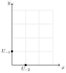
The recurrence \eqref{eq:recurrence} can be interpreted from a geometric perspective⁵. Corresponding to a rational number $\frac{p}{q}$ in reduced form we may may associate a point⁶ $(q,p) \in \mathbb{Z}^2$. Thus rather than ratios we have points. With regards to the recurrence \eqref{eq:recurrence}, we let $U_n$ denote the point $(q_n, p_n)$. Thus we have $U_{-2} = (1,0)$, $U_{-1} = (0,1)$, and \[ U_{n} = a_{n} U_{n-1} + U_{n-2}, \] where addition and scalar multiplication are componentwise.

Demonstration: Continued Fraction of 4/3

We illustrate this recurrence for the continued fraction expansion $[1,2,1]$ of $\frac{4}{3}$. To start, we have the points $U_{-2}$ and $U_{-1}$, shown below.

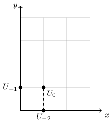
The point $U_0$ is given by the formula $U_0 = a_0 U_{-1} + U_{-2}$. This may be interpreted as follows: to get $U_0$, start at $U_{-2}$, and move $a_0$ multiples of $U_{-1}$. For us, $a_0 = 1$, which yields $U_0 = (1,1)$.

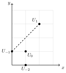
To obtain $U_1$, we proceed similarly: starting now at $U_{-1}$, we move $a_1 = 2$ multiples of $U_0$. Thus we have $U_1 = (2,3)$.

For the final iteration, start at $U_0$ and move by one ($a_2 = 1$) multiple of $U_1$, giving $U_2 = (3,4)$.

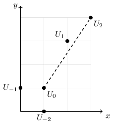
The three points $U_0,U_1,U_2$ correspond to the convergents $1$,$\frac{3}{2}$, and $\frac{4}{3}$ of $\frac{4}{3}$.

Properties of Convergents

One of the conveniences of this geometric view is that it makes apparent certain properties of the sequence of convergents. We list some of these below. All of these properties may be proved rigorously, and I make note of the corresponding theorems in Hardy and Wright’s book (see References).

First, note that the $x$ coordinate of the points $U_0,U_1,\ldots$ is strictly increasing. Recalling our notation $U_n = (q_n,p_n)$, this implies that the denominator $q_n$ in the convergent $\frac{p_n}{q_n}$ is strictly increasing. (HW, Theorems 155-156)
If we draw the line $y = \frac{4}{3}x$, the points $U_{-2}, U_{-1},\ldots$ are located on alternating sides of this line (at least, until the algorithm terminates).

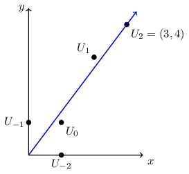
Indeed, the points with even indices are below the line, and the points with odd indices are above it. Considering another example, this time the continued fraction $\frac{8}{5} = [1,1,1,2]$, we again see this alternating pattern.

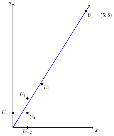
That the point $U_1 = (1,2)$ is above the line $y = \frac{8}{5}x$ implies that the convergent $\frac{p_1}{q_1} = 2$ is greater than $\frac{8}{5}$. Similarly, the convergent $\frac{p_2}{q_2} = \frac{3}{2}$ is less than $\frac{8}{5}$.
In addition to alternately lying above and below the line $y = \frac{4}{3}x$, the points $U_0,U_1,\ldots$ get successively closer to it. That is to say, as $n$ increases, the points $U_n = (q_n,p_n)$ get progressively closer to satisfying the equation $y = \frac{4}{3}x$ (a similar phenomena can be seen with the convergents of $\frac{8}{5}$, shown above). The error in the approximation $p_n \approx \frac{4}{3} q_n$ may be measured by \[ \Big| p_n - \frac{4}{3} q_n \Big|, \] or likewise \[ \Big| \frac{p_n}{q_n} - \frac{4}{3} \Big|. \]

There are in fact quantitative estimates for this error. We mention one general form: suppose $z = [a_0,a_1,\ldots,a_N]$. Then \[ \Big| z - \frac{p_n}{q_n} \Big| < \frac{1}{q_n^2}. \] (HW, Theorems 163-164)
Although it’s not as obvious, if one forms the triangles $OU_{n-1}U_n$, as shown below

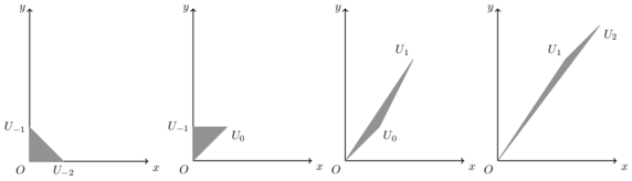
then it can be shown that, while these triangles grow longer and thinner, their area is always a constant $\frac{1}{2}$. This is tied up with one of the basic identities involving convergents, namely (HW, Theorem 150)
\begin{equation} p_n q_{n-1} - p_{n-1}q_n = (-1)^{n-1}. \label{eq:determinant} \end{equation}
The connection to triangles is then seen by writing \eqref{eq:determinant} as an identity involving determinants \[ \begin{vmatrix} q_{n-1} & q_n \\ p_{n-1} & p_n \end{vmatrix} = (-1)^{n-1}, \] and then noting that this determinant is the (signed) area of the parallelogram swept out by $U_{n-1}$ and $U_n$.⁷
The convergents $\frac{p_n}{q_n}$ are in reduced form. This is really not clear from the pictures, but follows easily from the identity \eqref{eq:determinant} since this implies that the $\gcd$ of $p_n$ and $q_n$ must be $1$. (HW, Theorem 157)

Existence and Uniqueness of Finite Continued Fraction Expansions

With the method we presented, it follows that any rational number $\frac{p}{q}$ may be represented by a finite, simple continued fraction $[a_0,a_1,\ldots,a_N]$. But is this representation unique?

Unfortately, no. There is one obvious source of non-uniqueness: the observation that $1 = \frac{1}{1}$. This means, for instance, that \[ \frac{7}{3} = [2,3] = [2,2,1]. \] More generally, if $a_N > 1$ we have \[ [a_0,a_1,\ldots,a_N] = [a_0,a_1,\ldots,a_N-1,1], \] and both of these are finite simple continued fractions. With that said, this is the only source of non-uniqueness. Indeed, we have the following theorem.

Any rational number can be expressed as a finite simple continued fraction in just two ways, one with an even and the other with an odd number of partial quotients. In one form the last partial quotient is 1, in the other is is greater than 1.

References

Hardy and Wright, An Introduction to the Theory of Numbers, 6th ed.
Stark, An Introduction to Number Theory.
Khinchin, Continued Fractions.

Footnotes

This approximation of $\pi$ is correct to six decimal places, whereas the naive alternative $\frac{314}{100}$ is only correct to two. It was known to the Chinese mathematician Zu Chongzhi.↩
Recall that (%), from Data.Ratio, constructs rational numbers.↩
The convenience of this will become apparent.↩
Actually, we left out one important thing. Given our definition of convergents, we need to ensure that $\frac{p_n}{q_n}$ is in reduced form. We take up this matter later.↩
This view is developed more fully in Harold Stark’s An Introduction to Number Theory.↩
Since we shall be adding points, and multiplying them by scalars, it would be appropriate to instead consider vectors. However, we do not make this distinction here.↩
When written in this matrix form, the fundamental recurrence for convergents is \[ \begin{pmatrix} q_{n-1} & q_n \\ p_{n-1} & p_n \end{pmatrix} = \begin{pmatrix} q_{n-2} & q_{n-1} \\ p_{n-2} & p_{n-1} \end{pmatrix} \begin{pmatrix} 0 & 1 \\ 1 & a_n \end{pmatrix}. \]↩