Braess' Paradox and the Price of Anarchy
A Routing Game
Consider the following scenario. A large number of independent agents wish to traverse a network, from some start vertex to some end vertex. Each edge they travel will take some time, which could in general depend on the number of agents traveling along the edge. For the sake of simplicity, we’ll normalize things so that \(x\) denotes a proportion of agents (i.e. \(x\) ranges from 0 to 1). In what follows, we will let \(\mathcal{E}\) denote the set of edges, and \(c_e : [0,1] \to \mathbb{R}\) the cost function associated with edge \(e\). A very simple example is something like the following, where \(s\) is the start and \(d\) is the destination, and edges have been labeled with their cost.
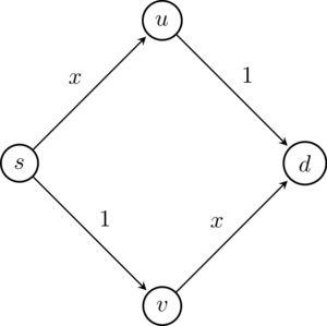
A simple routing network, with variable edge cost.
One way to summarize the entire set of paths chosen is via a flow \(f\), which assigns to each edge the normalized proportion of agents who have chosen to travel along it. For example, if all agents chose the top route in the above network, then we would have \(f_{su} = 1, f_{ud} = 1\) and \(f_{sv} = 0, f_{vd} = 0\). There are of course other possible flows; one could consider the flow that puts all agents along the bottom path, or another which mixes the top and bottom paths somehow. 1
For a general flow \(f\), the total cost borne by the agents in navigating the network is
\[ C(f) = \sum_{e \in E} f_e c_e(f_e). \]
In the above example, routing all traffic along the top path (or equivalently, the bottom path) has a total cost of \(2\). However, if one split the traffic so that half travels along the top path and half along the bottom path, then the total cost is only \(0.5 c_{su}(0.5) + 0.5 \cdot c_{ud} + 0.5 \cdot c_{sv}(0.5) + 0.5 \cdot_{vd}(0.5) = 1.5\). In this example, this turns out that this is the minimum cost flow. One could imagine that if we were benevolent dictators controlling the choices of the agents, we might opt for this as an outcome.
From an Agent’s Perspective
Another way of looking at this routing problem is from the agent’s point of view. Suppose that, for each path \(P\), some proportion of agents choose \(P\) for their traversal. In other words, we may imagine that we have a distribution \(g\) with \(g_P \geq 0\) and \(\sum_{P \in \mathcal{P}} g_P = 1\), where \(\mathcal{P}\) denotes the set of \(s-d\) paths through the network. Thus \(g_P\) is the proportion of agents choosing path \(P\). We’ll call such a \(g\) a path distribution, for lack of a better name.
There’s nothing lost by thinking about path distributions rather than flows. Indeed, given a path distribution \(g\) we can recover a flow by letting \(f_e = \sum_{P : e \in P} g_P\), where the sum is over all paths containing the edge \(e\). It’s not hard to show that this is an honest flow.2
So, from this vantage point: which path would an agent like to pick? In general, the cost of an edge depends on hhow much traffic it gets, so the answer is really contingent on the paths chosen by the other agents.
To give some clarity around this, let’s introduce an assumption about behavior: an agent will choose a path only if there are no cheaper alternatives. This is both a weak assumption, in the sense that it’s hard to argue with the rationale, and a strong one, in the sense that we’re granting each agent quite a lot of information about the problem at hand (e.g. the network topology, the behavior of the other agents, and so on).
With this in mind, note that relative to a fixed flow \(f\), the cost of a path \(P\) is
\[ C(P; f) = \sum_{e \in P} c_e(f_e). \]
Formally, a path distribution \(g\) is said to be a (pure Nash) equilibrium distribution if
\[ g_P > 0 \text{ only if } P \text{ minimizes } C(P; f), \]
where \(f\) is the flow associated with \(g\).
In other words, in an equilibrium distribution every agent takes a path that is minimal with respect to the flow induced by the others.
It’s worth mulling this over a bit. With an equilibrium distribution, there’s no incentive for any particular agent to switch paths. Each agent sees the social world around it as essentially fixed; the others have induced some flow \(f\), and the best one can do is pick the path that’s cheapest relative to this.
In our simple network, there is only one equilibrium distribution: half of the agents take the top path, and half take the bottom. The cost of this equilibrium distribution is \(1.5\), just as before.
Braess’ Paradox
To briefly recap, we’ve singled out two sorts of flows as being special.
- Cost-minimizing flows are the ones that we’d pick if were playing the part of a benevolent dictator.
- Equilibrium flows (i.e. those induced by an equilibrium path distribution) are the ones that we can imagine a bunch of independent agents settling for.
It was something of a coincidence that in our toy network these two ended up being the same. But they don’t have to be.
So what happens if we start adding edges to the network? Naively, it seems like it can only make things better. Certainly, adding an edge doesn’t increase the cost of any previous flows (since they simply do not use the new edge), and in fact it’s possible that it makes available a new, cheaper flow. So as benevolent dictators, there’s not much to lose.
But what happens when we think from the agent’s perspective? Surprisingly enough, adding an edge can shift the equilibrium flow to something even costlier! For an extreme example, consider adding a free edge to our previous network.
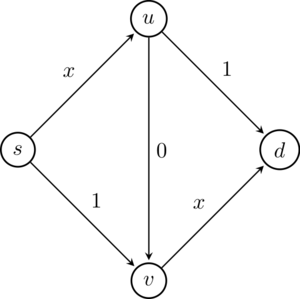
A network augmented with a zero cost edge.
With this addition, the equilibrium distribution 3 puts all of the agents on the path \(suvd\), for a total cost of 2! This is Braess’ paradox: adding capacity to a network can actually increase the cost of an equilibrium flow.
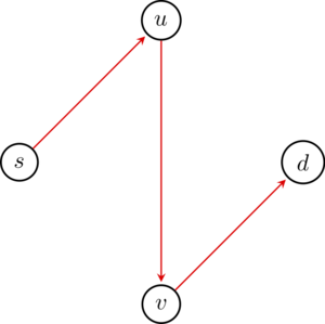
The new equilibrium flow.
I’m not going to prove that this flow is equilibrium, but let me give a glimpse of the incentives: the previous distribution, which put half of the agents on the top half and half of the agents on the bottom, is now unappealing from a traveller’s vantage point: relative to that flow, the effect of an agent on \(sud\) switching to \(suvd\) is to reduce their path cost by \(0.5\). And so on.
The Price of Anarchy
By definition, an equilibrium flow is at least as costly as a cost-minimizing flow. The ratio
\[ \frac{\text{maximum cost of an equilibrium flow}}{\text{cost of min cost flow}} \]
is sometimes referred to as the Price of Anarchy. For our original network, it was \(1\). After adding the edge, it was \(4/3\).
Footnotes
In general, a flow is a function \(f : E \to \mathbb{R}\) (where \(E\) is the set of edges), satisfying three conditions: i) sum of \(f\) on edges leaving \(s\) is 1, ii) the sum of \(f\) on edges entering \(d\) is 1, and iii) for any other vertex, the sum of \(f\) on incoming edges equals the sum of \(f\) on outgoing edges (i.e. the flow is ‘conserved’).↩
On the other hand, in a general network one might have several path distributions that induce the same flow.↩
In general, a routing game like this could have several equilibrium distributions. In this example, however, there is only one.↩